In our first post, we introduced the concept of manufacturing environments. In this post, we'll go into detail to define the different environments.
In a formal class I often lead with the question “Who Names the Environment?” and often received many different answers, including:
- Customers. They specify what they want and when they want it.
- Top management. They declare what it will be, and we must make it work out.
- Suppliers. They won’t change their lead-times because we are so small and have little power.
- Circumstance. The environment just happens to us. We do the best we can, but “stuff happens.”
Before continuing on, take a moment to stop to think what the answer would be for your company.
As we mentioned above, the name of the environment comes from the relationship between CLT and MLT:
Customer Lead-Time (CLT) |
The total length of time a customer is willing to wait for delivery of the item.
|
|
Manufacturing Lead-Time (MLT)
|
The total length of time it takes the selling organization to acquire all purchased items and produce the product to be ready for sale.
|
So, MLT has the longest cumulative lead-time. Cumulative MLT includes the longest lead-time at each level of the BOM, for both produced (make) and procured (buy) parts. Most ERP systems have a feature to calculate this time [1].
At a basic level, any time the cumulative MLT is longer than CLT, the result is inventory. Then, in order to plan for inventory at that level, a special system criterion appears. For example, a MTS company must have inventory at the top level of the BOM, often referred to as the FG level. In order to obtain FG inventory prior to customer orders arriving, they must forecast, or guess, what they are going to sell in a period of time so as to avoid a stock out. MTO organizations do not rely as much on a FG forecast.
The relationship between the CLT (demand) and the MLT (production) is sometimes referred to as the D:P ratio, where D = Demand and P = Production [2]. Please do not confuse the “DP” with Data Processing. This DP and that one are not the same thing. We will now explain the D:P ratio for each of the environments.
Make to Stock
The MTS environment is displayed on the graphic below. Note that there are two vertical lines next to the shape, one labeled MLT and one labeled CLT.
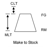
In the case of the MTS environment, the CLT is exaggerated as it extends above the top line of the shape. This indicates that the customer wanted it yesterday! In reality, MTS organizations often ship completed items within hours of receiving the order. To do so, the products are standardized. Standard means that every customer gets the same product and that there is little customization. By doing this, the company can keep stock “on the shelf” at the FG level with relatively low risk. If one customer does not buy the product, another may. There is no time to customize in the MTS environment. Just that little difference (i.e., customization) may move the environment to ATO.
On the graphic also note two other acronyms. At the top of the shape is FG. At the bottom is RM. The relationship between the two is defined in the Bills of Material (BOM). We will discuss these further in the next section.
Assemble to Order
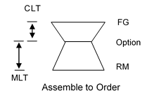
For ATO goods (shown below), the CLT extends from the top line of the shape to about the middle. This shows that the customer is willing to wait a little while for the product, but not the entire MLT. The customer is usually willing to wait a little longer for some degree of customization. This time can be a few hours to several months, depending on the product.
Dell ships completed computers, built to your specification from standard Sub-Assemblies (SA) within 24 hours of receiving your order. A manufacturer of farm equipment or specialty equipment (i.e., lift trucks) may take several weeks or months to deliver a product. In order to keep CLT manageable, interim SA and purchased material must be kept on hand and readily available. At Dell, every computer gets the same type and size of memory, hard drives, monitors, etc. These “option” level parts are stocked so that they can be assembled into your specific unit. The option level becomes standard inventory [3]. Standard means that every customer gets the same product and that there is little customization. When the customer order arrives, these items are assembled to customer requirements. Since every order is possibly different than any other order, stocking finished product would be a high risk for the producer.
In the ATO environment, we often find special modules (i.e., Configurator’s) to help manage the number of features and options. Features are logical groupings of types of parts (i.e., disk drives, memory, etc.). Options are the actual parts within those features (i.e., a 1 Terabyte hard drive, 2 Terabyte, etc.). In fact, there are so many combinations of features and options that the number of product configurations often approaches infinity very quickly. Two features, each with two options, results in 4 different combinations that could be assembled.
In the ATO environment, standard product moves from the FG level down to the sub-assembly level (i.e., material is stocked at the option level, not FG). In the MTO environment, it moves again from the sub-assembly to the raw material level (i.e., it is stocked close to the raw material level).
Make to Order
In the MTO environment (shown below), CLT is much longer than in the MTS or ATO environments. In fact, customers are willing to wait almost the entire MLT. Since every order is possibly different from any other order, stocking finished product would be a high risk. For this reason, in a MTO environment, production cannot be started until the customer order is received.
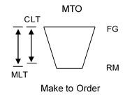
If any inventory is on hand in a MTO organization, it is near, or at, the bottom of the BOM. An example of this would be a company producing incinerators for the medical industry. While each incinerator is different, all are built from the same sizes and types of sheet steel. For the material, as long as steel is on hand (which can be a challenge due to lead-times and allocation in the steel market), then almost any incinerator can be produced without delays to the customer.
So, with a working description of each of the environments, who names them? In other words, who makes the decision on a product-by-product basis which operating environment to go with? The answer is based on the lead-times. The intersection of the CLT and MLT determines the environment. While we cannot control the CLT, we can control the MLT. Every decision made with respect to how many levels of a BOM, how to structure the shop floor for effective flow, etc. all add up to a lead-time. In other words, as managers we indirectly, or in some cases directly, affect lead-time and determine the environment. The sum of all management decisions, beginning with a declaration of what we are going to produce ultimately names the environment.
Before we move on, earlier we mentioned a fourth environment. The engineer to order (ETO) environment is basically the same as the MTO, except extra lead-time is needed to cover the design phase. The shape resembles that of a MTO. A good example would be the General Electric (GE) Space Division where orders are taken for space satellites for specific functions that have not been designed yet. Lead-times in ETO environments could be measured in months or years.
Engineer to Order
Before we move on, earlier we mentioned a fourth environment. The engineer to order (ETO) environment is basically the same as the MTO, except extra lead-time is needed to cover the design phase. The shape resembles that of a MTO. A good example would be the General Electric (GE) Space Division where orders are taken for space satellites for specific functions that have not been designed yet. Lead-times in ETO environments could be measured in months or years.
This is the second article in a multi-part series. You can visit part one here. Make sure to subscribe to our blog to stay up-to-date!
Ready to learn more right now? View our recorded webinar by clicking the image below:

Please let us know your thoughts or any questions below:
Footnotes
[1]In MAX – Sales Order Processing – Batch – Critical Path Lead-time, you can run an analysis on your Product Structure table for all parts, or simply your manufactured parts. The answer is stored in the Critical Path Lead-time field of the Part Master table. Furthermore, is System Configuration – Sales Order – Critical Path LT is set to “Y”, yes then the answer is also stored in the Critical Path Lead-time field of the Part Sales table. This number is then used to recommend the due date during sales order entry.
[2]For a good discussion of MLT vs. CLT see "Competitive Manufacturing", Hal Mather, Prentice Hall, 1988.
[3]These days (i.e., 2006), Dell may be buying the standard option parts from local suppliers that are stocking them for Dell. There are two lessons here: 1) As a customer, we don’t care where the inventory is located as long as we get the service we need, and 2) This discussion applies beyond the four walls of the factory and out to the extended supply chain.


